The problem
Many systems need to map one object to another, of the same or of a different type. This happens, for example, when they receive information in one form and want to convert it to another, or when they simply want to access information through a lightweight handle, called the key.
The family of data structures that does this is called associative containers, and they are fundamental in most modern systems. There are many ways to implement one, depending on what the system needs, but by far the most common is the hash table.
The main strength of hash tables is that all their operations are O(1) on average. That is why systems that care deeply about latency keep choosing them.
Trading systems are a typical low-latency application. In a trading system, a hash table could be used, for example, to map the number that uniquely identifies an order to the object that represents that order.
In fastbook, a low-latency market-data ingestion system, I use hash tables mainly for this reason. The lookup runs on almost every message the system receives from the exchange: when an order is added, executed or cancelled. It sits on the hot path, where every nanosecond matters and can make the difference between making and losing money. So the performance of these operations matters a lot, and, as we will see, while they are all O(1) in theory, in practice their cost differs by up to 6x depending on the implementation. Complexity analysis is very important when analyzing an algorithm or a data structure, but it is blind to several things that greatly affect real performance, even between two implementations with the same big-O complexity: cache misses, branch mispredictions, and data dependencies that destroy instruction-level parallelism.
In this post I measure and analyze four designs of associative containers that cover a wide range of trade-offs.
std::unordered_map
std::unordered_map is the associative container that ships with the C++ Standard Library.
It uses bucket chaining: when two keys land on the same slot of the array, their nodes are linked together in a linked list. This gives O(1) operations on average, but it does not use the capabilities of modern hardware very well.
The main reason is that traversing a linked list has terrible cache performance. The next pointers can point anywhere in memory, so the hardware prefetcher cannot learn a pattern and hide the latency of fetching the next node. The next node is also very likely not in the same 64 bytes (one cache line) as the current one, so every step can be a cache miss.
To make matters worse, the CPU pipeline also suffers, because every step is a data-dependent load (next = current->next). The next step cannot start early, because it needs the result of this load to know its address, so the CPU has to wait for each load to finish. This greatly limits instruction-level and memory-level parallelism (ILP/MLP) and leaves modern out-of-order processors underused.
Another issue with std::unordered_map is that every insertion and deletion goes through the allocator (new/delete), so its runtime behaviour is unpredictable and depends heavily on how the allocator is implemented. Some insertions get lucky, hit the allocator’s thread-local cache and get their memory quickly. In the worst case, an insertion ends up in the kernel (a system call or a page fault) and pays an unpredictable amount of latency for a single element.
std::map
std::map is the other associative container in the C++ Standard Library. Its operations are not O(1), but I decided to include it because I have seen many people reach for it. std::map keeps its key-value pairs sorted, and it pays O(log n) for that. This doesn’t sound too bad, but it is. std::map is a binary search tree, more specifically a red-black tree, a variant that keeps itself balanced. With 1.92M orders the tree is about 21 levels deep. And, make no mistake, every one of those levels is a dependent pointer load.
Cache performance is terrible here as well, for the same reasons as std::unordered_map. Nodes are linked through pointers that come from malloc, so they can be anywhere in memory and the hardware prefetcher is useless. std::map also pays a trip to the allocator for every node, but it is even worse than std::unordered_map, because a lookup walks about 20 nodes down the tree instead of one or two, and every insertion and deletion may also re-balance the tree, which writes to nodes all over it.
Linear probing
In fastbook, I needed an associative container mainly to map an order id to the Order object that describes that order. This hash table sits right on the hot path, so it needs to be as efficient as possible. For the reasons above (avoiding allocations, better use of the caches and the pipeline), I decided to implement my own. I built a simple linear probing hash table that stores the key-value pairs in contiguous, pre-allocated memory. I pre-fault all of that memory up front, so that no insertion or deletion on the hot path takes a page fault. A collision is resolved by probing the slots after the one that collided, until an empty one is found. Since the slots are contiguous in memory, this has excellent cache performance, for two reasons. First, the unit of transfer between caches is 64 bytes, one cache line. My slots are 16 bytes (an 8-byte key and an 8-byte pointer), so a cache line holds 4 of them, and 3 times out of 4 the next slot is already in the cache when the probe reaches it. This is one of the reasons I restricted the value to a pointer type (8 bytes). Second, the access pattern is sequential, which is the easiest pattern for the hardware prefetcher to follow. Linear probing hash tables have one tricky issue: what to do with deleted slots. You can’t just mark them as empty, because find() stops at an empty slot and could then miss valid entries further along. The common solution is to mark the slot as deleted (a tombstone) and step over it when searching. Another solution is to make erase() a bit more complex and move the following entries back, so that the deleted slot can be marked empty without breaking correctness. This also makes find() faster, since there are no tombstones to step over: when it meets an empty slot it stops right away and correctly concludes that the element is not present. I implemented both versions. The benchmarks below only show the backward-shift version. My tombstone version never cleans its tombstones up, so after enough erases there are almost no empty slots left, and every insert scans most of the table looking for a duplicate: around 18 µs per insert, against about 20 ns for finds and erases. On the real trading day it did not finish within my time limit.
SwissTable
While researching hash table designs that make good use of modern hardware, I came across SwissTable. Like linear probing, SwissTable stores its data contiguously, but it differs in a few ways. Next to the array that stores the key-value pairs, SwissTable keeps a second, parallel array with one control byte per slot. The byte says whether the slot is EMPTY or DELETED, and for a FULL slot it holds 7 bits of the key’s hash. A lookup compares those 7 bits first and only touches the key-value array when they match. Since each slot costs a single byte here, scanning this array has excellent cache performance: it takes the cache-line argument from linear probing to its extreme. Each 64-byte cache line now holds the state of 64 slots, which greatly improves the hit rate. On top of that, SwissTable uses SIMD, or SWAR (SIMD Within A Register), to compare several control bytes at once, which makes it two to three times faster than a simple scalar implementation, as we will see in the benchmarks. The details of how this is implemented can be found in the Swiss Tables design notes and in Matt Kulukundis’ CppCon 2017 talk, or in the source code of my implementation.
SwissTable also differs from linear probing in how it probes the table after a collision. It uses triangular probing instead of linear, which is guaranteed to visit every group when the capacity is a power of two. This way it tries to get the best of both worlds. It keeps what is good about linear probing, the cache locality inside a group, and it also reduces primary clustering. Primary clustering refers to the following phenomenon: With linear probing, a bad hash puts keys that collide next to each other, and later lookups may need many steps before they reach an empty slot, which hurts performance. With triangular probing, keys whose starting slots are close together end up more apart after the first group instead of getting merged into one long run.
Benchmarks
I benchmarked several variants of these implementations on a real workload: every order add, execute, cancel, delete and replace from a full NASDAQ trading day (the ITCH capture of 30 December 2019), turned into 289M inserts, finds and erases on order ids. At peak time, 1.92M orders were live at the same time.
The variants are:
- Linear probing (the backward-shift version)
- SwissTable with SSE2 (128-bit) SIMD: 16 control bytes at a time
- SwissTable with AVX2 (256-bit) SIMD: 32 control bytes at a time
- SwissTable with SWAR (plain 64-bit integer instructions): 8 control bytes at a time
- SwissTable with a scalar loop: 1 control byte at a time
- std::unordered_map
- std::map
Linear probing and SwissTable get the same memory: two slots per live order at the peak (4M slots, a 64 MiB table, never more than 46% full). std::unordered_map reserves its buckets up front.
The experiments ran on a rented bare-metal machine with the following specifications:
Machine
- Hetzner AX41, bare metal: AMD Ryzen 5 3600 (Zen 2), 6 cores, SMT off.
- Caches: 32 KiB L1d and 512 KiB L2 per core, and 16 MiB of L3 shared by each group of 3 cores.
- 64 GB DDR4-2400. Linux 7.0, gcc 15.2,
-O3 -mavx2.
Setup. The benchmark is single-threaded and pinned to core 3.
- Core 3 runs nothing else:
- no other tasks (
isolcpus) - no timer tick (
nohz_full) - no kernel RCU callbacks (
rcu_nocbs) - no interrupts (all IRQs routed to core 0)
- no other tasks (
- Clock Frequency: 3.6 GHz with boost off.
- Profiling: I used profiling.hpp, the small profiling library I built for fastbook.
- Latency: every operation is timed on its own, with
rdtscpfollowed bylfenceon both sides, so the CPU cannot move any of the operation’s work outside the two reads. - Histograms: each latency goes into a log-linear histogram. Every power-of-two range is split into 16 bins and a percentile is reported as the upper edge of its bin. Two latencies that land in the same bin show up as exactly the same number.
- Hardware counters: read with the
perf_event_openAPI right before and right after the measured loop, in a separate run with no timing inside the loop.
- Latency: every operation is timed on its own, with
A full trading day
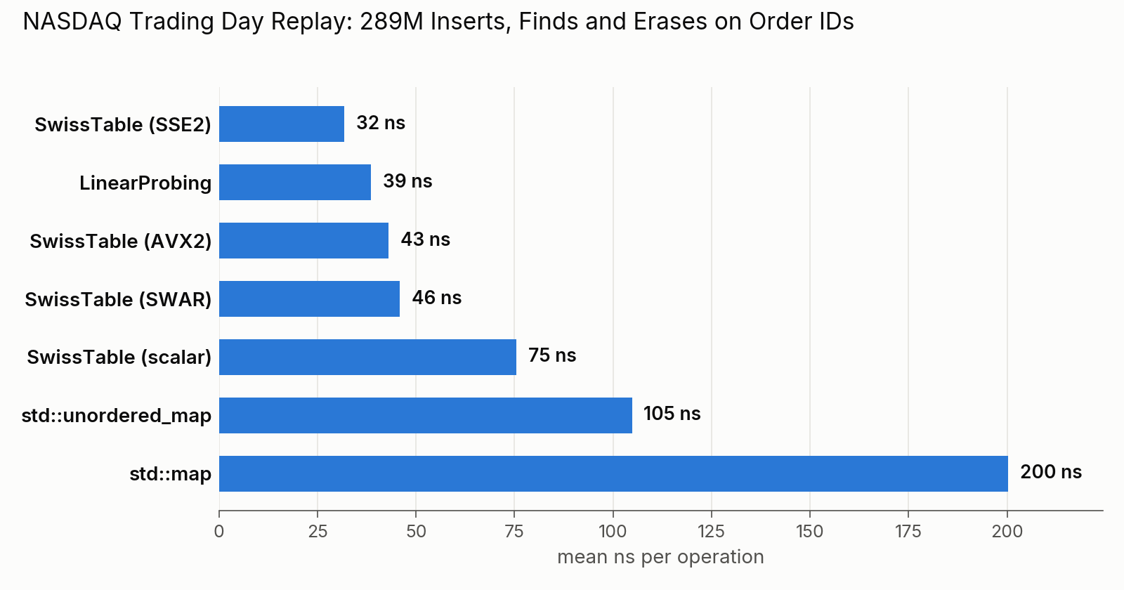
In this plot we can clearly see the benefit of the open-addressing hash tables over the bucket chaining of std::unordered_map and the red-black tree of std::map, for the reasons mentioned above. The hardware counters further below show where exactly the difference comes from.
One interesting takeaway from this plot is that linear probing, despite having no SIMD and despite the clustering problems that come with it, is the second best implementation. This came as a surprise to me. Looking at the behaviour and the hardware counters, I can see two reasons why:
First, linear probing keeps key and value together in one 16-byte slot (4 of them fit in a cache line), so an operation usually touches one cache line. SwissTable touches two separate arrays: first the control bytes, then the slot.
This table clearly shows:
| per operation | LinearProbing | SwissTable (SSE2) | SwissTable (AVX2) |
|---|---|---|---|
| loads served from L3 | 0.44 | 1.34 | 1.52 |
| dTLB misses | 0.94 | 1.84 | 1.84 |
| instructions | 57 | 73 | 99 |
In short: at this size the workload is memory-bound, and linear probing touches fewer cache lines per operation.
Second, clustering, the main weakness of linear probing, barely shows up here. The tables have ~4M slots and at most 1.92M entries were live at once, so they were never more than half full. The probes stay short, and since a cache line holds 4 slots, a probe rarely leaves the line it started in.
SSE2 still wins, and it wins on inserts. It finds a free slot by scanning the control bytes (about 4 MiB in total, so they most likely stay in L3), and then it only writes the slot, which the CPU does not have to wait for. Linear probing has to read the slot from DRAM first, to see that it is empty. This shows up in the counters: SSE2 touches more cache lines in total, but most of the extra ones are control bytes that come from L3, which is cheap. It goes to DRAM, the expensive part, less often than linear probing (0.55 vs 0.64 loads per operation), and in the end needs fewer cycles (114 vs 139).
Table size vs. cache size
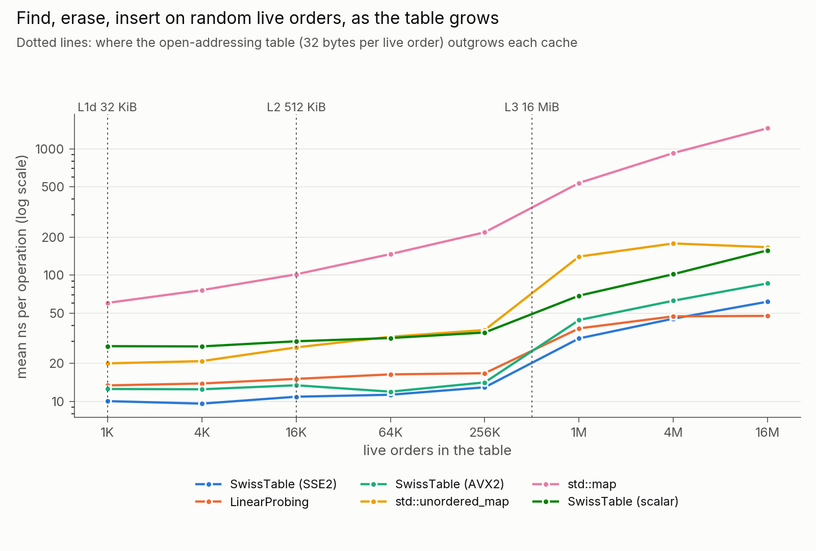
Unlike the trading day, this experiment uses a synthetic workload, since the real day has a fixed size. The table always holds the same number of live orders, and every step finds a random live order, erases another random one and inserts a new one. So finds, erases and inserts are around 1/3 each, while the real day is about 48% inserts, 48% erases and 3% finds. This plot shows how performance changes as the table stops fitting in each level of cache. std::map and std::unordered_map get much worse once the table outgrows the caches: from 1K to 16M live orders, std::map goes from 60 to 1,457 ns per operation (24x) and std::unordered_map from 20 to 166 ns (8x). This is the cost of dependent loads and pointer chasing, which the prefetcher cannot hide. The SIMD versions of SwissTable are the fastest up to 4M live orders, because the control-byte array is small and fits in the caches. But at 16M orders, linear probing beats every SwissTable variant (48 vs 62 ns for SSE2). At that size the control bytes alone are 32 MiB and no longer fit in the 16 MiB L3, so SwissTable pays for two DRAM misses per operation (control byte, then slot), while linear probing finds the key and the value in the same slot and touches less memory overall.
Where the cycles go
Hardware counters per operation on the real trading day, with the operations running back to back:
| Container | cycles/op | instructions/op | loads from L2/op | loads from L3/op | loads from DRAM/op | dTLB misses/op | page faults |
|---|---|---|---|---|---|---|---|
| SwissTable (SSE2) | 114 | 73 | 0.22 | 1.34 | 0.55 | 1.84 | 0 |
| LinearProbing | 139 | 57 | 0.10 | 0.44 | 0.64 | 0.94 | 0 |
| SwissTable (AVX2) | 155 | 99 | 0.22 | 1.52 | 0.57 | 1.84 | 0 |
| SwissTable (SWAR) | 164 | 115 | 0.22 | 1.37 | 0.55 | 1.86 | 6 |
| SwissTable (scalar) | 271 | 350 | 0.21 | 1.29 | 0.55 | 1.84 | 0 |
| std::unordered_map | 377 | 121 | 0.60 | 1.28 | 0.95 | 2.65 | 15,030 |
| std::map | 719 | 405 | 4.33 | 3.68 | 0.54 | 17.12 | 30,062 |
Key takeaways:
- The workload is memory-bound. Every row except scalar SwissTable has an IPC (instructions per cycle) below 1, which means the CPU spends most of its time waiting for data, not executing instructions.
- The open-addressing tables go to DRAM about equally often (0.55 to 0.64 loads per operation). Linear probing has far fewer L3 loads and TLB misses, because it keeps everything in one array. SwissTable reads two arrays and pays for it with more memory traffic. This is the main trade-off between the two designs.
- The SIMD effect is crystal clear in the instructions column (scalar 350 → SWAR 115 → SSE2 73) and in the cycles column (271 → 164 → 114). Interestingly, AVX2 loses to SSE2 in both. The tables are less than half full, so the first 16 slots almost always already contain the answer (the key or an empty slot) and scanning 32 bytes is mostly wasted work. A 32-byte load also crosses a cache-line boundary about twice as often as a 16-byte one, which shows up as more L3 loads (1.52 vs 1.34). Wider SIMD is not always faster.
- Page faults are another big difference between my tables and the STL containers. Because I control the allocation and pre-fault the memory at start-up, my tables take (almost) no page faults during the run, while the STL containers take 15k–30k as they grow, each one a trip to the kernel on the hot path. This is one of the reasons why low-latency code bases keep STL containers off the hot path, or give them custom allocators.
When the table fits in L3, the simplest table wins
This table shows the latency of a single operation when the table fits in the 16 MiB L3, using the synthetic workload from the size sweep with 262,144 live orders (an 8 MiB table). Each operation is timed separately.
| Container | mean | p50 | p99 | p99.9 |
|---|---|---|---|---|
| LinearProbing | 30 ns | 31 ns | 102 ns | 142 ns |
| SwissTable (SSE2) | 34 ns | 31 ns | 111 ns | 204 ns |
| SwissTable (AVX2) | 35 ns | 31 ns | 62 ns | 124 ns |
| SwissTable (SWAR) | 37 ns | 31 ns | 111 ns | 142 ns |
| SwissTable (scalar) | 50 ns | 51 ns | 133 ns | 204 ns |
| std::unordered_map | 69 ns | 71 ns | 178 ns | 498 ns |
| std::map | 252 ns | 266 ns | 746 ns | 995 ns |
Keep in mind that the time-stamp counter moves in steps of about 10 ns, and that every percentile is the upper end of the histogram bin (see Profiling above). Tables whose latencies land in the same bin show exactly the same number, which is why several p50s are identical. The mean does not have this problem, because the 10 ns steps average out over millions of operations.
Interestingly, once the table fits in L3 and we are no longer DRAM-bound, linear probing has the lowest mean latency (30 vs 34 ns for SwissTable SSE2). It touches fewer cache lines, and without DRAM misses to hide behind, the SIMD scan doesn’t buy as much.
Looking at the tail, AVX2 does best (p99 of 62 ns). My guess is that its 32-slot window covers, in one step, the cases where a 16-slot window is full and the probe has to move on to the next group, while linear probing occasionally pays for a longer probe. For the STL containers we can clearly see the effects of pointer chasing and allocation: up to 8x worse than the best table.
Conclusion
Associative containers are everywhere, and in low-latency systems they need to be as fast as possible. I implemented, benchmarked and analyzed several of them to understand the trade-offs of each one. As always in software, there is no clear winner for every workload: SwissTable SSE2 was the fastest on the real trading day, while linear probing won once the table fit in L3, and again once it far outgrew it. The right choice depends on the size of the working set compared to the caches, the access pattern and how full the table gets. And that is why the main rule about performance is to never guess about performance.